Trajectory forecasting models aim to predict the future positions of agents given past observations. However, many real-world applications such as sports analytics require not just prediction, but controllable simulation of plausible futures under hypothetical scenarios. In this post, I investigate diffusion-based models for trajectory generation, and show how high-level “sketches” of plays can guide multi-agent dynamics. I have open sourced the code base for the model and canvas app.
1. The idea of sketch-guided trajectory simulation
During NBA games, coaches often have to plan attacking plays to break through a defensive setup within a short period of time. They may sketch out instructions for a few players on a whiteboard, and rely on their mental model to project how both teammates and opponents might move in response. Prior work has explored data-driven approaches for this problem, using imitation learning1 and GANs2 to generate sketch-conditioned gameplay simulations. In this post, I explore whether diffusion models3 4 can be used for this task as well. If you are unfamiliar with diffusion, please check out this post.
2. Why diffusion for this task
Previously, I got good results modeling trajectory prediction with an autoregressive setup5. One intuition I had was that autoregressive models effectively get more compute capacity per sample compared to most parallel prediction models of similar size, as each step requires a new forward pass and reuses the full model capacity. In practice, this often leads to more coherent trajectories.
Diffusion models share a similar property. Instead of generating trajectories in a single pass, they can iteratively refine a noisy sample over multiple forward passes, repeatedly applying their full capacity in the process.
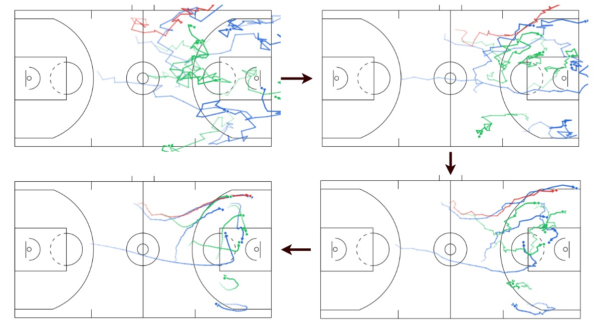
Progressive denoising of a sampled gameplay from my model. The overall structure of the play (spacing and movement direction) emerges earlier, with later steps refining finer details.
I later came across interpretations of diffusion as a form of autoregression in the frequency domain6, which further supports this connection. This planted the idea in my head that diffusion models could be a viable alternative for trajectory simulation. The key difference is that diffusion models operate on the full trajectory jointly at every refinement step, allowing them to repeatedly adjust the entire trajectory in a globally consistent way. In contrast, autoregressive models, even with access to global context, are structured around a sequential generation process. This makes it less natural to use that context for satisfying global or future constraints.
One simple example is when we want to guide only part of a play at a few future time points. In the diffusion setup, this can be expressed directly as partial conditioning at those time points, even if intermediate frames are missing. The model then refines the full trajectory to approximately satisfy these constraints. In contrast, autoregressive models commit to predictions step-by-step and tend to prioritize local consistency. This makes it harder to guide the sample trajectory towards matching a future endpoint, without modifying the generation process.
3. Model setup
Instead of generating absolute positions, I decide to make the model generate frame-to-frame position deltas for each agent. This keeps the target distribution more uniform in scale and makes the learning problem easier, especially for longer trajectories. The model operates on tensors of shape: [batch, seq_len, num_agents, coord_dim].
Model backbone
The overall architecture is inspired by DiT7, but adapted for sequential multi-agent data rather than images. The key design choice is to factorize attention across time and agents, rather than applying joint attention over all dimensions. Concretely, we alternate between two types of transformer layers:
- Temporal attention layers, which attend over the temporal dimension independently for each agent
- Agent attention layers, which attend over all agents at each fixed timestep
This factorization allows the model to separately capture temporal dynamics (how trajectories evolve) and inter-agent interactions (coordination, collision avoidance), without paying the full cost of joint attention over all dimensions. Conceptually, this is similar to spatiotemporal factorization used in video models (e.g. within Genie8), where attention is separated along spatial and temporal axes.
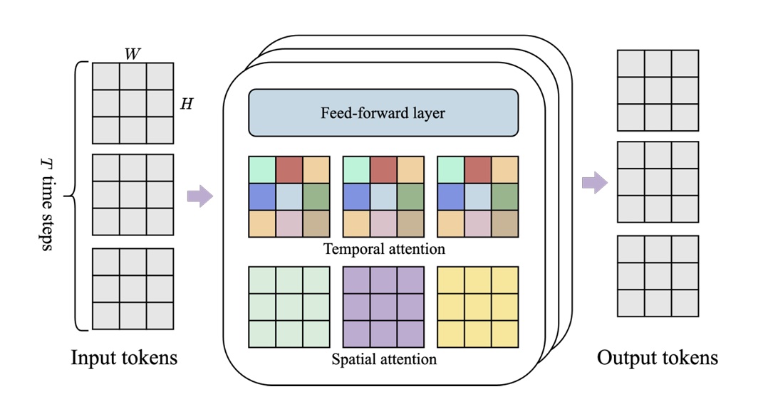
Spatiotemporal module used in the Genie model, with interleaved spatial and temporal attention layers. Each color represents a single self attention map: spatial layer attends all spatial locations over the image at one timepoint, temporal layer attends one spatial location over time. (Image source: Bruce, J., et al. 2024).
In our setup, we make a small adaptation from the original DiT design by creating patches along the time dimension for each agent, reflecting the sequential nature of the data.
Applying conditioning
For conditioning, we provide trajectories and its stepwise deltas (with observed + mask-filled portions) and a binary mask of the same shape indicating which values are actually observed. This allows us to flexibly specify partial observations or sketch-based constraints.
I experimented with classifier-free guidance (CFG)9 to control the strength of conditioning during sampling. In this setting, I found it to be quite sensitive. One possible reason is that the unconditional branch is relatively noisy. Since we parameterize the generation target as trajectory deltas, the dynamics are highly dependent on anchor points such as agent positions at specific time points provided in the context. Without such minimal reference, the unconditional model has to represent a very broad distribution over possible trajectories, which can make it a poor baseline. Since CFG scales the difference between conditional and unconditional predictions, this can lead to unstable guidance signals and distorted trajectories when the guidance scale is increased. Empirically, values around \(gs = 1.0\) produced the most coherent results. I’ll defer a deeper discussion of how CFG works to a separate post, and highly recommend this post10 for an intuitive understanding.
Other stuff
The model is trained using a noise-prediction diffusion objective with learned variance parameterization. For readers who are interested about the implementation details, please refer to the code base.
4. Sanity check benchmark
Before diving deeper into sketch-guided simulation, I wanted to sanity check whether the model can handle a standard trajectory forecasting setup. I follow a common protocol on an NBA trajectory dataset from SportVU, where the first 2 seconds of player and ball movements are treated as observed trajectories, and the task is to predict their positions over the next 4 seconds. In my setup, I just need to treat the first 2 seconds’ data as conditioning input.
minADE\(_{20}\) / minFDE\(_{20}\) (metres) results:
| Time | GroupNet11 CVPR'22 |
LED12 CVPR'23 |
MoFlow (joint obj.) |
MoFlow13 CVPR'25 |
CausalTraj5 (C-PointNet) |
This Work |
|---|---|---|---|---|---|---|
| 1.0s | 0.25/0.32 | 0.21/0.27 | 0.28/0.39 | 0.18/0.25 | 0.15/0.21 | 0.17/0.22 |
| 2.0s | 0.47/0.68 | 0.44/0.56 | 0.48/0.71 | 0.34/0.47 | 0.34/0.50 | 0.35/0.51 |
| 3.0s | 0.71/0.99 | 0.69/0.84 | 0.68/1.01 | 0.52/0.67 | 0.55/0.78 | 0.57/0.79 |
| 4.0s | 0.95/1.22 | 0.81/1.10 | 0.89/1.32 | 0.71/0.87 | 0.77/1.01 | 0.79/1.03 |
minJADE\(_{20}\) / minJFDE\(_{20}\) (metres) results:
| Time | GroupNet CVPR'22 |
LED CVPR'23 |
MoFlow (joint obj.) |
MoFlow CVPR'25 |
CausalTraj (C-PointNet) |
This Work |
|---|---|---|---|---|---|---|
| 1.0s | 0.50/0.77 | 0.34/0.64 | 0.40/0.67 | 0.37/0.68 | 0.28/0.50 | 0.27/0.52 |
| 2.0s | 1.04/1.91 | 0.78/1.55 | 0.81/1.61 | 0.80/1.61 | 0.62/1.18 | 0.64/1.21 |
| 3.0s | 1.61/2.98 | 1.22/2.36 | 1.27/2.55 | 1.25/2.49 | 0.98/1.86 | 1.01/1.89 |
| 4.0s | 2.12/3.72 | 1.63/2.99 | 1.72/3.33 | 1.69/3.31 | 1.34/2.47 | 1.36/2.47 |
The ADE and FDE metrics measure the average and final displacement error of predicted trajectories against the ground truth. Specifically, they report the minimum error over 20 candidate future trajectories, selected independently for each agent. The joint metrics (minJADE, minJFDE) instead require selecting a single candidate trajectory jointly for all agents, without mixing predictions across different candidates. The lower the values the better. I haven’t spent much time tuning hyperparameters yet and this model is already performing competitively with prior work.
Also, as the default ancestral sampling method is too time-consuming, we resort to using DPM-Solver++14 for accelerated sampling to produce the results in this benchmark. This is expected to sacrifice the performance a little as we do not make use of the learned variance during sampling. I will make another post in the future to go into more details about several accelerated sampling methods for diffusion.
5. From canvas to simulation
I made a simple gameplay trajectory canvas app with streamlit so that it is convenient for anyone to create guidance trajectory sketches to feed to the model.
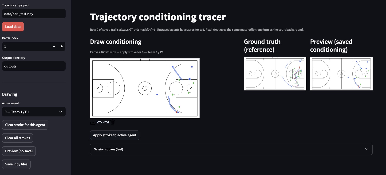
You can fire up the app and load the dataset locally. You can simply select an active agent on the left, then use your cursor to sketch out the path you want the agent to follow in the next 6 seconds on the court.
For now, the conditioning interface is still quite minimal. The sketched trajectories are converted into paths with a fixed time horizon, and I currently assume a uniform speed along the path. This is obviously a simplification, and it limits the expressiveness of the instructions. In reality, player movement often involves changes in speed, pauses, and more nuanced intent.
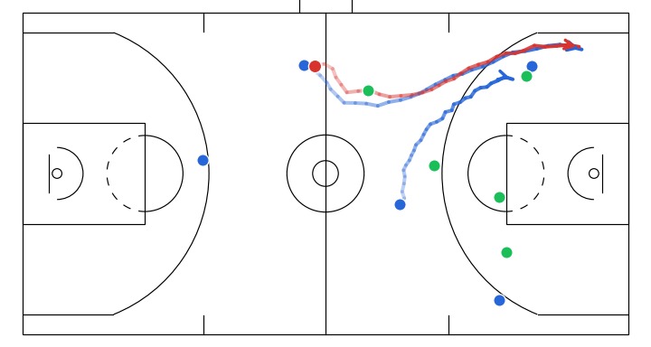
Here I will show a few instructive sketches I made with the app given the same initial game state, and their corresponding simulations generated by the model:
- Off-ball interchange between 2 attackers to stir up defense structure.
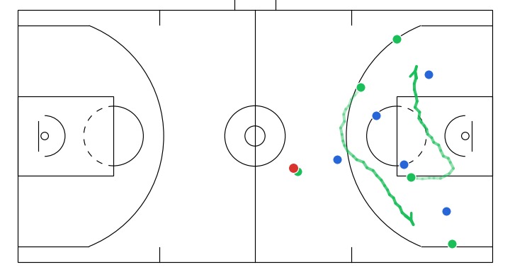

- A player attempts a screen to free the ball handler for a drive.
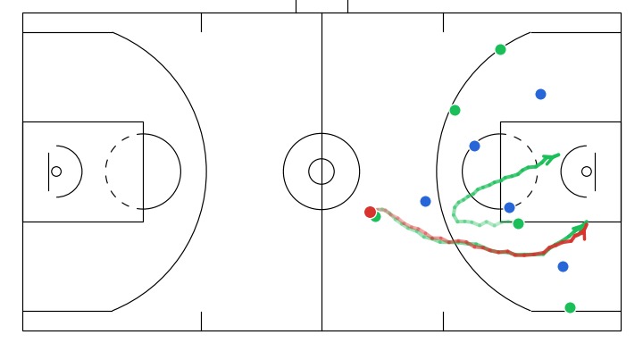
- A dribble handoff between the initial dribbler and the player on the right.


6. Takeaways and next steps
Diffusion models are pretty flexible when it comes to conditioning. You can guide them with partial trajectory inputs at different time points, even with different temporal extents for each agent. Denoising behaves as a form of global, progressive refinement, where high-level structure of the play emerges earlier and finer details are resolved over time, compared with the strictly sequential prediction in autoregressive models.
Moving forward, I think we absolutely need better ways to evaluate simulation quality, including both realism (how plausible the trajectories are) and controllability (how well the outputs follow the given instructions). I also intend to explore richer forms of control, such as allowing users to specify speed profiles, or even higher-level instructions (e.g. “move into this area within the next few seconds”) instead of requiring a fully specified trajectory.
If you spotted any errors in this post or have ideas that you would like to discuss, please leave a comment!
If you would like to cite this post in an academic context, you can use the following BibTeX:
@misc{teoh2026trajectorydiffusion,
  author       = {Teoh, Wei Zhen},
  title        = {Diffusion for Sketch-Guided Trajectory Simulation},
  year         = {2026},
  url          = {https://wezteoh.github.io/posts/diffusion-for-sketch-guided-trajectory-simulation},
  note         = {Technical blog post}
}
References
-
Seidl, T., Cherukumudi, A., Hartnett, A., Carr, P., & Lucey, P. (2018). Bhostgusters: Realtime interactive play sketching with synthesized NBA defenses. MIT Sloan Sports Analytics Conference. https://www.sloansportsconference.com/research-papers/bhostgusters-realtime-interactive-play-sketching-with-synthesized-nba-defenses ↩︎
-
Hsieh, H.-Y., Chen, C.-Y., Wang, Y.-S., & Chuang, J.-H. (2019). BasketballGAN: Generating basketball play simulation through sketching. arXiv. https://arxiv.org/abs/1909.07088 ↩︎
-
Sohl-Dickstein, J., Weiss, E. A., Maheswaranathan, N., & Ganguli, S. (2015). Deep unsupervised learning using nonequilibrium thermodynamics. arXiv. https://arxiv.org/abs/1503.03585 ↩︎
-
Ho, J., Jain, A., & Abbeel, P. (2020). Denoising diffusion probabilistic models. arXiv:2006.11239 ↩︎
-
Teoh, W. Z. (2025). Coherent multi-agent trajectory forecasting in team sports with CausalTraj. arXiv. https://arxiv.org/abs/2511.18248 ↩︎ ↩︎
-
Dieleman, S. (2024, September 2). Diffusion is spectral autoregression. https://sander.ai/2024/09/02/spectral-autoregression.html ↩︎
-
Peebles, W., & Xie, S. (2022). Scalable diffusion models with transformers. arXiv preprint arXiv:2212.09748. https://arxiv.org/abs/2212.09748 ↩︎
-
Bruce, J., et al. (2024). Genie: Generative interactive environments. arXiv. https://arxiv.org/abs/2402.15391 ↩︎
-
Ho, J., & Salimans, T. (2022). Classifier-free diffusion guidance. arXiv. https://arxiv.org/abs/2207.12598 ↩︎
-
Dieleman, S. (2022, May 26). Guidance: A cheat code for diffusion models. https://sander.ai/2022/05/26/guidance.html ↩︎
-
Xu, C., Li, M., Ni, Z., Zhang, Y., & Chen, S. (2022). GroupNet: Multiscale hypergraph neural networks for trajectory prediction with relational reasoning. arXiv. https://arxiv.org/abs/2204.08770 ↩︎
-
Mao, W., Xu, C., Zhu, Q., Chen, S., & Wang, Y. (2023). Leapfrog diffusion model for stochastic trajectory prediction. arXiv. https://arxiv.org/abs/2303.10895 ↩︎
-
Fu, Y., Yan, Q., Wang, L., Li, K., & Liao, R. (2025). MoFlow: One-step flow matching for human trajectory forecasting via implicit maximum likelihood estimation based distillation. arXiv. https://arxiv.org/abs/2503.09950 ↩︎
-
Lu, C., Zhou, Y., Bao, F., Chen, J., Li, C., & Zhu, J. (2022). DPM-Solver++: Fast solver for guided sampling of diffusion probabilistic models. arXiv. http://arxiv.org/abs/2211.01095 ↩︎